ABSTRACT
To be reliably operated off-shore wind turbines need an assured downtime and maintenance pattern to keep costs low. A monitoring project carried out by the authors uses an infrared (LWIR) thermal camera placed in the drive trains of such turbines and focusing on their spherical roller bearings. A bearing having an inner raceway fault shows a faster and higher temperature increase than a healthy bearing. Whereas vibrations tend to propagate through the drive train, temperature increase is a more local phenomenon. The article presents a methodology for analyzing such measurements based on a thermal camera for the detection, visualization and localization of faults. This makes it a promising tool in the condition monitoring of fully covered and sealed rolling element bearings in industrial applications.
Introduction
Short-termed maintenance of wind turbines on high seas is very expensive. Replacing faulty components can take months. Thus, early and reliable fault detection can avoid more expensive consequential damage, or even a complete failure leading to loss of production. Figure 1 outlines the main components of a gearbox-based wind turbine drive train. Due to their tribological nature gears and bearings are affected by wear and friction. Consequences include vibration, acoustic and heat emissions, which can be monitored by different sensor-based techniques. The main cause of downtime are faults in the drive train, with bearing faults belonging to the major reliability issues, because bearings must deal with cyclic and transient loads as well as alignment problems. The majority of gearbox faults in wind turbines appear to originate in the bearings and propagate towards the gear teeth.
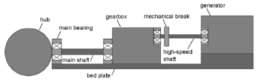
Figure 1. Wind turbine drive train with gearbox.
Vibrations and acoustic emissions propagate through the drive train structure, which can make fault localization difficult. It requires great expertise and detailed system models. Real-time oil analysis is usually limited to measuring oil quality and particle counts. To obtain more detailed information for identifying the faulty component and a fault classification requires an on-shore sample analysis, which itself can be costly regarding time and financing. Most bearing faults result in increased temperature. This offers the opportunity of using thermal imaging for a real-time monitoring and localization. It also allows a spatial visualization of the heat propagation in the monitored areas. Increased temperature is usually a more local phenomenon, so thermal imaging can improve fault detection and complement the currently used condition monitoring techniques. A multiple-sensor approach combining classic techniques such as vibration analysis with thermal imaging is a promising alternative for early fault detection, on-line component identification and real-time fault classification.
Experimental Setup
The test setup shown in Figure 2 was used for monitoring FAG 22205-E1-K spherical roller bearings. As seen in Figure 4, these bearings consist of cylindrical rollers, which manage high axial forces oscillating in both directions, as well as radial forces. They are designed to handle heavy loads such as in wind turbines. The close oscillation between rollers and raceways supports uniform stress distribution. The bearings are completely covered and sealed. In this setup, the bearings were mounted within FAG SNV052-F-L plummer block housings. The shaft is a solid Cf53, made of hardened and ground steel, and has a diameter of 20 mm with an h6 tolerance rate.
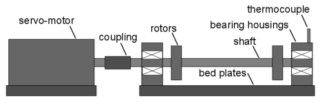
Figure 2. Scheme of the test setup
Besides intact bearings, intentionally pre-damaged bearings were monitored as well. Pitting, as one of the most common faults with a variety of possible causes, was simulated by means of a milling machine. Figure 3 shows small holes of a triangular shape that were added to the outer ring of a bearing. The same kind of fault was added to the inner ring of another bearing.

Figure 3. Intentionally pre-damaged outer raceway
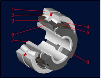
Figure 4. 3D scheme of spherical roller bearing
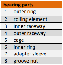
Table 1. Spherical roller bearing parts
Each of these tests ran for one hour at a speed of 1,500 rotations per minute, which is standard for high-speed components in European wind turbine drive trains. To monitor the setup, the Gobi-640-GigE, an uncooled long-wave infrared (LWIR) camera by Xenics, was used at 6.25 frames/sec (Figure 5). The thermocouples located behind the setup are to monitor the ambient temperature, which serves as reference for the data processing. Figure 5.

Figure 5. Uncooled long-wave infrared (LWIR) camera Gobi-640 made by Xenics
Methodology
Thermal measurements were performed for both healthy and faulty bearings. Before each measurement, the setup was cooled down to ambient temperature in order to receive a comparable starting situation and to understand the general heat-up process. All bearings were monitored from various points of view. Our analysis is focusing on the camera location sideways of the setup. This allows the monitoring of both bearing housing and shaft, as indicated in Figures 6 and 7. This view is most promising for monitoring the effects of outer raceway faults, as well as inner raceway faults. Figure 7 is a thermal image taken from the side of the housing for the healthy bearing after a measurement period of sixty minutes. Because the bearing housing and the shaft exhibit different temperature characteristics and noise effects, reflections and regions of interests were selected and further analyzed. Both two-dimensional and three-dimensional surface plots were analyzed to determine the actual thermal characteristics of both healthy and faulty bearings as well as noise, to consequently support the choice of meaningful regions of interest.
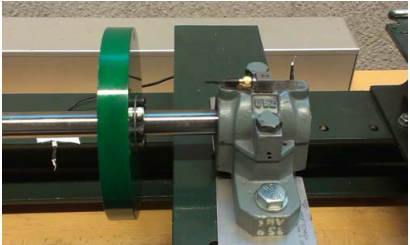
Figure 6. Bearing housing and shaft from the side
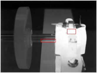
Figure 7. Thermal image of bearing housing and shaft with regions of interest
The upper housing is closest to the outer ring because of lower material thickness and is therefore selected as the first region of interest. The bottom part of the shaft next to the bearing housing is expected to show a heat increase based on both natural impacts such as shaft bending as well as bearing faults. Therefore it was selected as second region of interest. To reduce the impact of environmental changes, all diagrams show the temperature relative to ambient temperature. In other words, the ambient temperature is subtracted from the absolute temperature.
Ambient temperature is measured by the thermocouples seen in the back of the setup in Figure 6. Using relative temperatures instead of absolute temperatures yields consistent results independent of ambient temperature. This procedure significantly reduces step effects in the trend graphs caused by camera calibration. It therefore improves the readability of the data.
For each bearing, four measurements were performed with the discussed camera location. Inner raceway faults consistently show higher temperatures than healthy bearings, as well as faster temperature increases. However, the difference of the maximum temperatures between both bearings at the end of each measurement varies. Therefore, average trends are created from four individual measurements for each bearing.
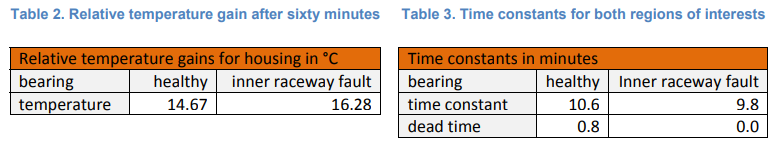
Furthermore, both the temperature gain and the time constants are discussed for these average trends. Relative temperature gain is the difference between the relative temperatures of the system in non-operating state, and after sixty minutes in the operating state. To get the time constants, the trend graphs of both the healthy bearing and the inner raceway fault are matched with first-order dynamics. The time constant of the system response is the time required by the step response to reach 63% of its final value.
Results
This methodology is applied to both healthy and faulty bearings. First, the surfaces of both bearing housing and shaft are analyzed to determine regions of interests for trend analysis. Each of the presented surface plots displays the last image taken at the end of the corresponding measurement period of sixty minutes.
Frame-wise analysis of bearing housing
Figure 8 shows how the non-uniform surface of the bearing housing leads to different temperature characteristics. The material of the upper housing is thinner and tends to a faster heat-increase than the bottom part. The screw visible in the upper center of the housing as well as the polished surface on top of the housing cause distinct drops in the measurements, making these regions unsuitable for further analysis. The central upper region of the housing is closest to the outer bearing ring because of thinner material and shows the highest temperatures. Therefore, this region is chosen for further analysis.
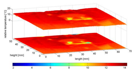
Figure 8. Three-dimensional surface plot of the housing of a healthy bearing.
The region of interest for the healthy bearing is shown in Figure 9 and for the bearing with inner raceway fault in Figure 10. As both images show noise caused by reflection of light, the thermal measurements need to be carefully analyzed. For the inner raceway fault, higher temperatures are monitored as well as stronger heat propagation across the surface, which is indicated by the more uniform color representation.
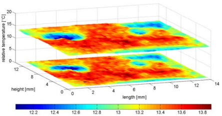
Figure 9. Housing region of interest for a healthy bearing.
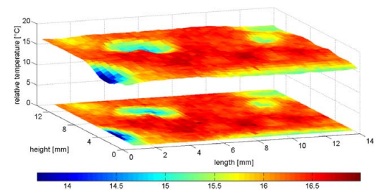
Figure 10. Housing region of interest for a bearing with inner raceway fault.
Frame-wise analysis of the shaft.
The second region of interest is the shaft. Increased temperatures were encountered in the bottom right shaft next to the bearing housing. This becomes more distinct in the surface plots in Figures 11 and 12. They represent the complete shaft part between bearing housing and mass rotor for both healthy and faulty bearings.
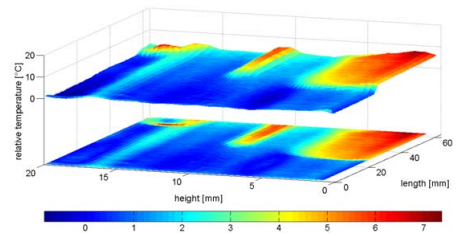
Figure 11. Three-dimensional surface plot of shaft in a side view for healthy bearing.

Figure 12. Three-dimensional surface plot of a shaft in side view for an inner raceway fault.
The shaft shows a distinct heat increase next to the bearing housing for both healthy and faulty bearings. As the housing is sealed and the rotation of the shaft seems to provide a cooling effect, this heat increase only occurs in a small region. Central and upper shaft regions show lower temperatures and in fact no distinguishable heat increase for both healthy and faulty bearings. The peaks in the upper shaft are caused by light reflections. It is evident that the locations of the reflections on the shaft are not fixed but slightly oscillating up and down. Because of these characteristics, a further analysis of the shaft focuses on the heat increase in the bottom part next to the housing.
Trend analysis
The surface plots shown give insight in the temperature distribution in the regions of interest at a
specific point in time, or more precise: after sixty minutes of system runtime. Whereas the region of interest at the housing shows a more uniform temperature distribution, the shaft is strongly affected by the light reflection. A significant heat increase is seen only in its bottom right corner, next to the bearing housing.However, a first trend analysis of the shaft did not permit a reliable distinction between healthy and faulty bearings. Therefore, the trend analysis focuses on the region of interest in the upper center of the housing. The central point of this region, which is not affected by light reflection, is selected for the following trend analysis. Figures 13 and 14 show the average relative temperature increases and step responses for the central point of the region of interest on the housing, independent of the ambient temperature. Whereas the thermocouples indicate only small differences in the ambient temperature, the temperature of the housing clearly differs for the various bearings. In particular, the temperature of an inner raceway fault increases faster than in the healthy bearing.
The inner raceway fault follows a first-order behavior straight from the beginning. The healthy bearing shows a more second-order behavior. Second-order behavior is approximated by a first-order model with dead time. The dead time defines the initial time required by the trend to show first-order behavior. In particular, a dead time of 48 seconds is determined for the healthy bearing.
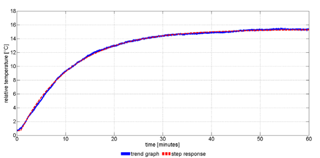
Figure 13. Relative temperature trend and step response of the housing in a healthy bearing.
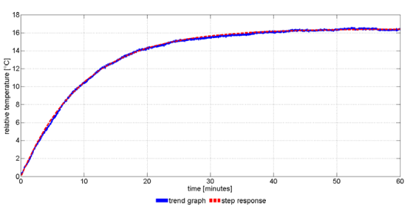
Figure 14. Relative temperature trend and step response of the housing for a bearing with inner raceway fault.
Table 2 lists the relative temperature gains of the housing for both healthy and faulty bearings after sixty minutes. Table 3 shows the time constants for a temperature increase of both healthy and faulty bearing. The stronger temperature gain and faster heat increase in the bearing with an inner raceway fault enable a distinction between healthy and faulty bearings. They also reveal the potential for fault detection by thermal imaging.
Conclusion
Fully covered and sealed rolling element bearings monitored by a thermal camera show different temperature increases in a healthy bearing and a bearing with inner raceway fault. The inner raceway fault leads to a faster and higher temperature increase of the housing. Whereas vibrations propagate through the drive train and fault localization requires high expertise, temperature increase is of a more local impact as can be seen in the temperature propagation from the housing towards the shaft. Thermal cameras are useful for visualizing as well as localizing faults as a promising tool for condition monitoring of wind turbine drive trains.
References
[1] Entezami M., Hillmansen S., Roberts C., “Distributed Fault Detection and Diagnosis for Wind Farms”, Annual
Conference of the Prognostics and Health Management Society, Portland (USA), 2010
[2] Costinas S., Diaconescu I., Fagarasanu I., “Wind Power Plant Condition Monitoring”, 3rd WSEAS International Conference on Energy Planning, Energy Saving, Environmental Education, Tenerife (Spain), 2009
[3] Daneshi-Far Z., Capolino G.A., Henao H., “Review of Failures and Condition Monitoring in Wind Turbine Generators”. XIX International Conference on Electrical Machines, Rome (Italy) 2010. [4] Kusiak A., Verma A., “Prediction of Status Patterns of Wind Turbines: A Data Mining Approach”. Journal of Solar Energy Engineering, vol. 133, American Society of Mechanical Engineers, New York (USA), 2011. [5] Hannon W.M., “Rolling Bearing Condition Monitoring”, Encyclopedia of Tribology, pp. 2812-2820, Springer Science+Business Media, New York (USA), 2013 [6] Kang, Y.S., “Rolling Bearing Contact Fatigue”, Encyclopedia of Tribology, pp. 2820-2824, Springer
Science+Business Media, New York (USA), 2013 [7] Sheng S., Veers P., “Wind Turbine Drivetrain Condition Monitoring” Applied Systems Health Conference, Virginia Beach (USA), 2011. [8] Lu B., Li Y., Wu X., Yang Z., “A Review of Recent Advances in Wind Turbine Condition Monitoring and Fault Diagnosis”, IEEE Power Electronics and Machines in Wind Applications, Lincoln (USA), 2009 [9] Terrell E.J., Needelman W.M., Kyle J.P., “Wind Turbine Tribology”. Green Tribology – Biomimetics, Energy Conservation and Sustainability, pp. 483-530, Springer International Publishing, Cham (Switzerland), 2012. [10] Musial W., Butterfield S., “Improving Wind Turbine Gearbox Reliability”. European Wind Energy Conference, Milan (Italy), 2007 [11] Zhang Z., Verma A., Kusiak A., “Fault Analysis and Condition Monitoring of the Wind Turbine Gearbox”, IEEE Transactions on Energy Conversion, Vol. 27, No. 2, pp. 526-535, 2012 [12] Hannon W.M., Houpert L., “Rolling Bearing Heat Transfer and Temperature”, Encyclopedia of Tribology, pp. 2831-2839, Springer Science+Business Media, New York (USA), 2013 [13] Tavner P.J., “Review of condition monitoring of rotating electrical machines”, IET Electric Power Applications, Vol. 2, No. 4, pp. 215-247, 2008 [14] García Márquez F.P., Tobias A.M., Pinar Pérez J.M., Papaelias M., “Condition Monitoring for Wind Turbines: Techniques and Methods”, Renewable Energy, Vol. 46, pp. 169-178, 2012 [15] Nise N.S., “Control Systems Engineering”, 6th Edition, pp. 166-168, John Wiley & Sons (Asia), Singapore, 2011
Documentation
Application Note


Related content

Jul 22nd 2026
Cooled and Uncooled Infrared Cameras :
Infrared cameras have become essential tools across a wide range of industries, from defense and surveillance to industrial inspection.

Munich.
FROM Nov 10th 2026 TO Nov 13th 2026
SEMICON EUROPA 2026
Join Exosens at SEMICON EUROPA 2026 2026 in Munich

Edinburgh.
FROM Sep 14th 2026 TO Sep 17th 2026
SPIE Sensors + Imaging 2026
Join Exosens at SPIE Sensors + Imaging 2026 Edinburgh, United Kingdom

Jul 07th 2026
Multifocal Femtosecond Laser Writing
Crosstalk Limits in Multifocal Parallel Femtosecond Direct Laser Writing: Decoherence Strategies and Quantitative Validation of Nanostructure Optical Phase

Jun 29th 2026
Exosens secures contract with BROLIS
Exosens secures major long-term contract with BROLIS to supply 17000 high-performance image intensifier tubes for the Czech Armed Forces

Aug 20th 2021
Visit our booth #514 during OPTIFAB

Jun 25th 2026
Strengthening Defense & Security Innovation
Exosens secures €140 million in EIB financing to foster innovation in Europe’s defense and security industry